Prediction of ultrafast Laser flashes.
This is a quick summary of my paper published here. Check it out if you are interested in the details!
What is an X-ray Free Electron Laser (XFEL)?
Motivation for XFELs
X-ray free electron lasers are some of the largest machines used for research today. The two biggest ones are LCLS in Stanford, California and euXFEL in Hamburg, Germany. Each spans multiple kilometres in length, at a similar scale as the large hadron collider (LHC) at CERN (albeit a bit smaller).
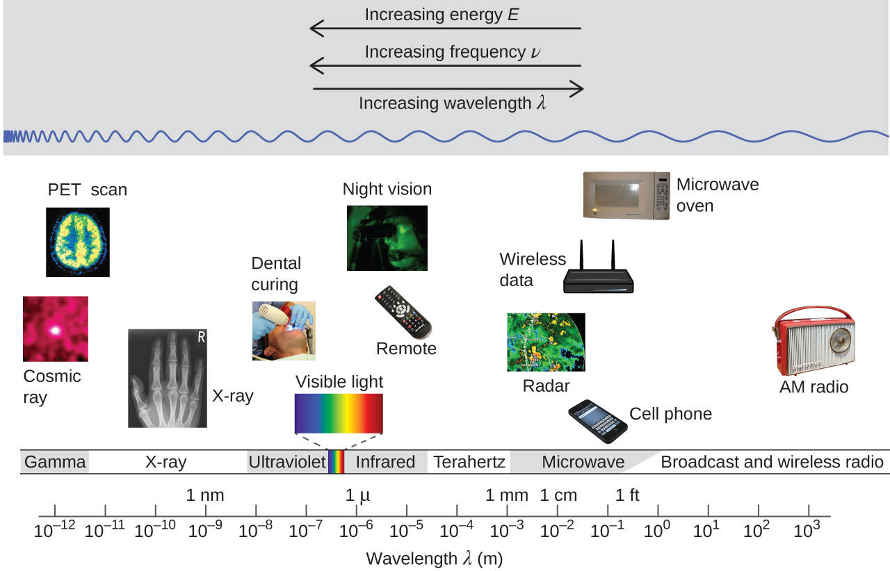
They are capable of generating very short, very bright laser flashes at regular intervals. This alone makes them very useful for investigations into ultrafast processes in diverse fields. However, they also provide the benefit of reaching parts of the electromagnetic spectrum that no other Laser source is capable of: the hard X-ray regime.
These properties motivated the development of XFELs, but these huge machines have their own drawbacks. To understand what exactly the challenges of using an XFEL are, we need to first understand how they work.
Inner workings of an XFEL
To dissect what an XFEL is, it’s useful to begin with the name itself: X-ray Free Electron Laser. We now know that it’s a Laser that generates X-rays, so those components of the acronym are clear. But where do the free electrons come in?
Remember that we compared XFELs to the large hadron collider, probably the most famous particle accelerator in the world? That was no coincidence. Indeed, every XFEL is built around a particle accelerator. The two main differences are:
- XFEL accelerators are usually linear accelerators (LINACs), whereas the LHC is a circular accelerator.
- XFELs rely on the acceleration of electrons, whereas LHC accelerates protons.
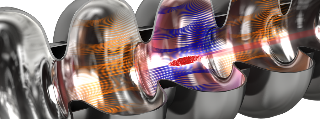
The “Free Electrons” in XFEL are those that are being accelerated! They are usually generated in bunches from an electrode, and then accelerated using so-called radiofrequency (RF) cavities. Each cavity contains an electric field that will push the electrons and, if timed correctly, the electrons keep accelerating through all of them. If the timing is off, the electrons can instead be pushed back by a cavity, causing them to slow down. As the electrons travel through a tube that contains a vacuum, they collide with nothing and can be accelerated to very close to the speed of light. This speed is important for generating the laser, because XFELs rely on the electrons being able to keep up with any light that’s emitted.
Once the electrons are fast enough, they are passed through sets of strong magnets with alternating directions, called either undulators or wigglers, depending on how much humour you have. Why are they called that? Well… they wiggle the electrons around. Due to the Lorentz force, the electrons will be made to accelerate first in one direction and then the other in short succession, leading to a wiggly trajectory.
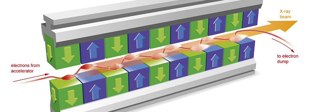
This gives rise to another effect: charged particles that experience acceleration emit light (electromagnetic radiation if we are being technical). This so-called synchrotron radiation is at the core of a lot of research facilities. XFELs are set up so that the emitted light is in the X-ray part of the spectrum and points in the same direction that the electron beam travels in.
This is where the really weird part happens. Because the electrons are so fast, they travel alongside the light which is only ever so slightly faster. Now, light can be described as consisting of electric and magnetic field waves which in turn exert a force on the electrons. This causes the electron bunch to separate into so-called micro-bunches, which are aligned with the wavelength of the light. This alignment leads to the electrons amplifying light at the energy that corresponds to their spacing, and with the right phase to generate (quasi-)coherent light. The reasons for this are complicated, and well outside the scope of this post. The important part is that this process, called self-amplified spontaneous emission (SASE), is what generates the laser pulses.
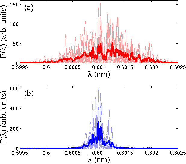
Now, I have made a slight simplification by only talking about “the light”, as if all light emitted is the same. Unfortunately, this isn’t the case. Instead, the initial emission of light occurs across a range of frequencies, and which of them happens to become dominant and strongly amplified is essentially random. The effect of this is a very spiky spectrum, with each spike corresponding to an amplified frequency. These spikes are superimposed on a wider base of frequencies that occur, leading to the spectra shown below.
Why do we need to predict XFEL pulses?
Pulse shapes & repetition rates
The complex shape of these spectra, and their bandwidth spanning multiple electron volts in energy, make them difficult to use in experiments, despite all the favourable properties XFELs exhibit. To still make use of these pulses, we need to know what they look like1. The easiest way of doing so, is by pointing a camera at the pulse. However, that suddenly becomes a problem if we want to use the pulse for something else (like an actual experiment). There are ways around such a destructive measurement scheme, usually by splitting off part of the beam and redirecting it to a camera, while the remainder of the beam continues on to the experiment. Another issue, however, persists to this day with this approach: Cameras are slow. While XFELs have historically generated flashes at no more than 60 Hz or so (about the same rate as most monitors update their image), there has recently been a push towards faster operation to make more use out of existing XFELs. At LCLS, this has come in the form of LCLS-II, while the European XFEL has been capable of operating at 1,000s of shots per second for a while.
These frequencies are pushing the boundaries of both measurement devices and data infrastructure, giving us an incentive to reduce the amount of measurements (especially expensive and relatively slow imaging) that is to be undertaken. This is the backdrop for a work by Sanchez-Gonzalez et al. in which they use neural networks to predict pulse energies and timings for a so-called slotted foil two-pulse mode. This was highly successful, with excellent predictions being obtained on data collected from LCLS. Unfortunately, the slotted-foil mode itself has some drawbacks, which lead to the development of other setups for two-colour modes.
So, can machine learning be leveraged to predict pulse properties of these newer modes?
Results
The short answer: Yes!
The slightly longer answer: Yes, but…
The full answer:
Yes, it can. However, it seems that there are some key differences in the modes, that we don’t fully understand yet. What we can tell is that the quality of predictions is unfortunately lower than that seen in Sanchez-Gonzalez et al. We validated that this has nothing to do with a difference in data analysis routines by applying our code to both the newer data, and that used by Sanchez-Gonzalez et al. The difference in performance was significant, and our work matched the prior results well.
We combined this comparison with some additional analysis on the performance of machine learning, and which features really contribute to pulse predictions. The full work can be read here. The key results are that:
- Only a handful of input data (features) make up the vast majority of predictive capability, and we don’t need the others.
- Very different models perform equally well, indicating that we are limited by data quality and not model choice.
- Depending on the exact configuration of our XFEL setup, we can actually make predictions with increased or reduced accuracy.
Now, let’s unpack these one by one!
Feature Importance
Anyone familiar with machine learning will know the term “feature”, but for those that are new to the subject, I will give a quick introduction:
A feature is the data that you put into a machine learning model. It then returns a prediction to you. This prediction is compared to the so-called label, which is the data that you use to check how well your model is performing.
Now, in most machine learning applications, you might have a model giving great predictions, but you have no idea why. One of the most common ways of trying to understand the reasons for why a model is performing well, is called permutation feature importance.
Essentially, once you have trained a model, you can investigate how each individual feature impacts predictions, by shuffling (or permuting) them one at a time. If the prediction quality drops significantly for a feature being shuffled, that will be deemed a predictive feature. If on the other hand shuffling a feature has virtually no effect on predictions, it is likely non-predictive. Note that there is an exception to this rule in the case of highly correlated features. If I have two features with high correlation, my estimator may (depending on the original random seeds) randomly pick one of them to use as a predictor, and largely ignore the other. If this is the case, the feature that hasn’t been picked can show up with a low permutation feature importance, but may actually act as a useful predictor if the model is trained once more with a different initialization.
Overall, this process will give us a ranking of the importance for each feature. We can then use this ranking to retrain an estimator using only the top x features, where we increase the value of x starting from 1 until the quality of predictions (on the test set) once again matches that of the estimator using all features. In our case, this analysis demonstrated that only 10 of an original set of 300+ features actually aid in the prediction. The others were unnecessary data, which might even incentivize model overfitting if used in combination with a very powerful model.
This was a useful result, as reducing data overhead can aid in allowing for faster operational modes on XFELs.
Model Choice
We used three different models:
- A simple linear model
- Gradient boosted decision trees (learn more about them here)
- Feed forward neural networks
Models 2 & 3 were also optimized with regard to hyperparameters (parameters that are fixed before any machine learning happens, and that need to be varied manually).
Our results show that both the gradient boosted decision trees and the neural networks perform equally well on the experimental data. The quality of predictions is also notably worse than those seen in other experiments. Finally, we also applied all methods to these other experiments, and obtained much better predictions, indicating conclusively that the correlation of the experimental features and labels was the issue, rather than the chosen machine learning approach.
XFEL Configuration
Finally, we found some interesting results relating to predictive quality depending on the experimental configuration with regard to the two-colour mode. The details of this are quite technical, so I recommend you check out the original article or contact me directly if you are interested in this aspect of our work.
Methods
For a detailed description of our methods, check out the paper here!
If you are more interested in the code, you can check that out here.
-
Technically, we can also use seeding or a monochromator, but they come with their own downsides, a discussion of which is outside the scope of this post. ↩