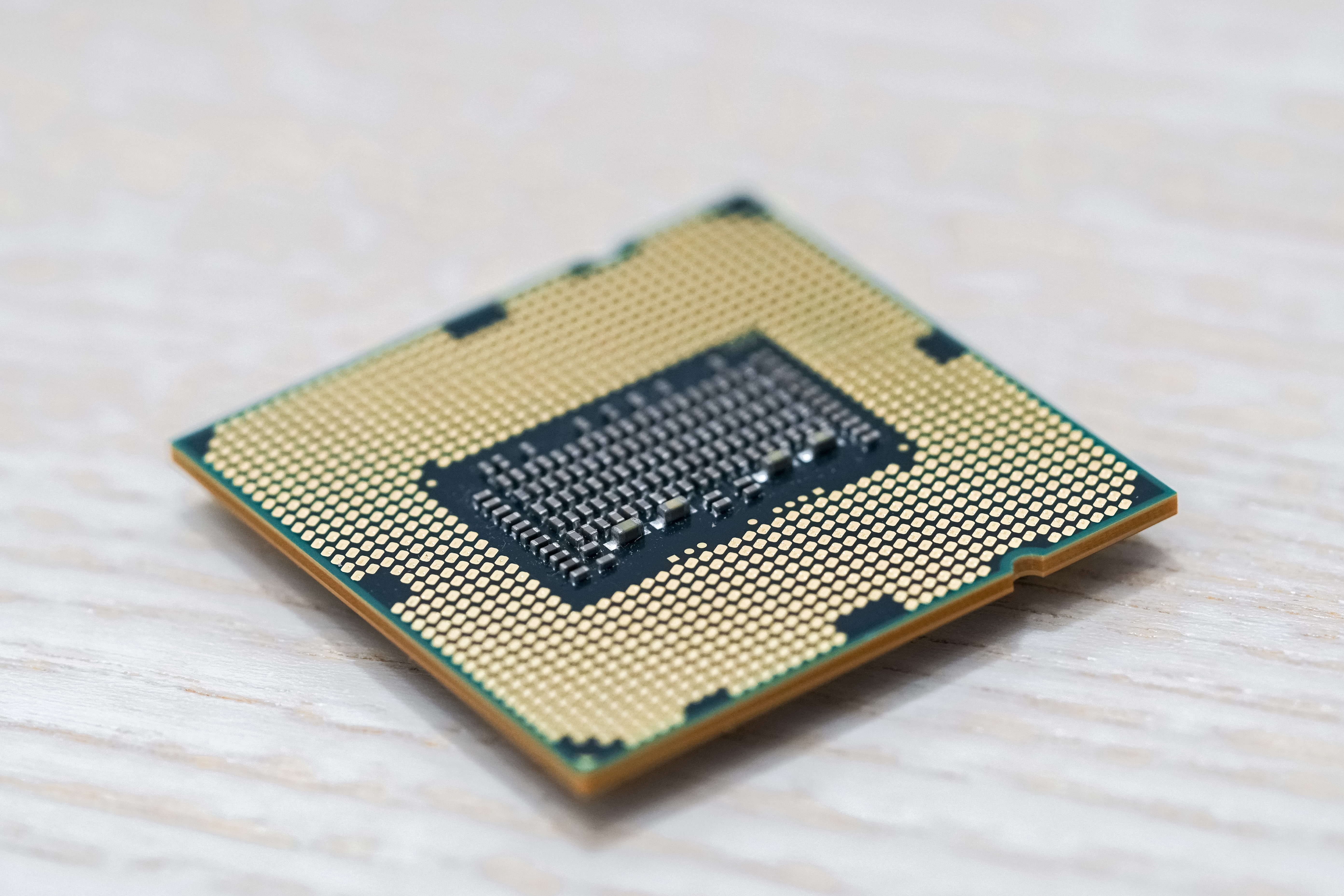
CPU-Simulation

This is the source code that was created for my 2020 Computational Physics module Project (Project 4). It can be used to simulate the temperature in a CPU with different configurations for Heat Sinks and convection cooling. For any questions or requests, contact me.

The separation into subfolders was intended, but made counterproductive by pythons default behaviour regarding imports.

The report for this can be found here.

DISCLAIMER: The issue with figures not showing up during runtime is known. See "Troubleshooting" for more information.

Dependencies

The project was written in python 3.8 and requires new features available from it to run. It was developed in the anaconda 3 environment using spyder 4. The project has only been tested under Windows 10, but should run reliably there.

It furthermore requires the following python packages: numpy matplotlib time (standard package) abc (standard package) dataclasses (standard package) unittest (standard package)

If any of these are not installed, you can install them with either:

pip install packagename

or if you are using anaconda:

conda install packagename

Running the Code

In order to run the code, you can use the prepackaged interface from main.py, which is used to reproduce all of the actual results presented in the results section of the project report. They should be sufficient for default systems with the same material specifications as in the aforementioned report. This includes:

main() wrapper function that handles dynamic user input -> This is the easiest entrypoint, others can be called from here

run_presets() function, which runs all of the presets plotted in the report (huge, slow system is optional)

run_system() function to model any system with default materials and settings

optimise() function to perform grid search over specified heat sink parameter ranges

calls to the test_all() function (see "Tests and Validations" below)

Here, the NewtonSolver is used exclusively as the ExactSolver and RelaxationSolver are deprecated (See manual systems or tests and validations for their usage).

Troubleshooting

If the figures do not appear when running from the main loop function, this is due to matplotlib not rendering while the loop runs. For this, either call the functions directly and not from the loop, or simply terminate the loop (not python, just exit the loop as intended) and the plots will appear.

Tests and Validations

Files for testing and validation of all the functions and classes are included in the package (under test_file.py). These can be used to extensively test not only the base behaviour of methods and classes, but also their agreement etc. The exact test files are:

test_linalg.py (For manual linear algebra solver self-consistency and agreement with numpy.linalg solver)
test_system.py (For proper system setup and not taking invalid parameters)
test_method.py (For testing of proper setup and agreement of the different methods (ExactSolver, RelaxationSolver and NewtonSolver))
test_resolution.py (For testing insignificant improvements for resolutions larger than 2)
vboundaries.py (For testing the differences between the two boundary condition schemes: forward- and central-difference)

testing.py (For running all of the tests consecutively)

The tests can also all be run from the main.py file through the test_all() function from testing.py

Manual System Creation

Alternatively, completely custom systems can be set up very easily by following these steps:

Define all of you materials through the Material Dataclass from system.py: Air, the Processor, Case, and optionally the Heat Sink. (Custom parameters for power and conductivity can be passed)
Group these materials in a list of length 3 (without heat sink) or 4 (with heat sink).
(Optional) create a heat sink, either with 10 fins, 2mm apart and 20mm long each or pass custom parameters for these features.
Initialise and name your system through the System dataclass from system.py. Choose a resolution (minimum 2) This automatically creates a layout, which can be called with the show() method on the dataclass.
Choose your parameters (Convection mode, Boundary Condition option, manual or numpy linear algebra solver and possibly forced convection wind speed) and call your preferred solver.Here, there are the following options:
```
 ExactSolver (deprecated, only works for Forward-Difference-Scheme BCs and Forced convection)
 RelaxationSolver (deprecated, slow)

 NewtonSolver (preferred in all cases)
```
These all automatically initialise a heat map and generate all the linear algebra equations required for solving the equations. You can also use the show() method on them to plot a heat map.
Finally call solve() method on your Solver, where you can choose from the list of parameters, which linear algebra to use, which error to use as the convergence criterion etc. (See help(YourChosenSolver.solve))